Guidelines are presented to better understand the temperature profiles of high-velocity gases
 In high-velocity gas flows, such as those that may occur within the discharge piping of a pressure-relief or depressurization valve, the temperature experienced at the wall of the pipe through which the gas is flowing can be much higher than the flowing stream’s “static” temperature. In fact, the wall temperature approaches the stagnation temperature, which is the temperature that would be obtained if the fluid were brought adiabatically and reversibly (isentropically) to rest.
Experimental work in aeronautical engineering has established this effective adiabatic wall temperature, and correlations have been proposed to determine the “recovery factor” as a function of the Prandtl number (Pr) of the fluid. It has been found that the adiabatic wall temperature is about 90% of the difference between the stagnation and static temperatures for a turbulent gas having a Prandtl number of 0.7, which is typical for many gases. When performing heat-transfer calculations between the pipe and the gas, or when specifying temperatures for piping material selection, this recovery factor is important, and should be accounted for.
Recent investigations into the potential for fluid temperatures to exist below the embrittlement temperature of relief-valve discharge piping have shown that low-flowing temperatures can exist for a wide variety of systems, including: flashing liquids or two-phase flow; autorefrigeration and Joule-Thompson cooling in response to pressure drops; and high-velocity gas flow [1].
There is evidence that some systems exhibiting these behaviors have resulted in metal embrittlement and failure. However, there is an apparent lack of evidence supporting embrittlement failures involving high-velocity gas flow, and there is some suspicion that the flowing temperatures experienced in high-velocity gas flow may not be realistic, as evidenced by a common refrain — “if the gas was getting this cold, I would be seeing ice on the pipes.” Some attempt to reconcile this anecdotal evidence with the “intuition” that the pipe (or vessel) wall temperature can approach the bulk fluid temperature given a long enough pipe and a low enough convective loss to ambient from the pipe is needed. This article provides guidance in determining the wall temperature for high-velocity gas systems.
Boundary layers
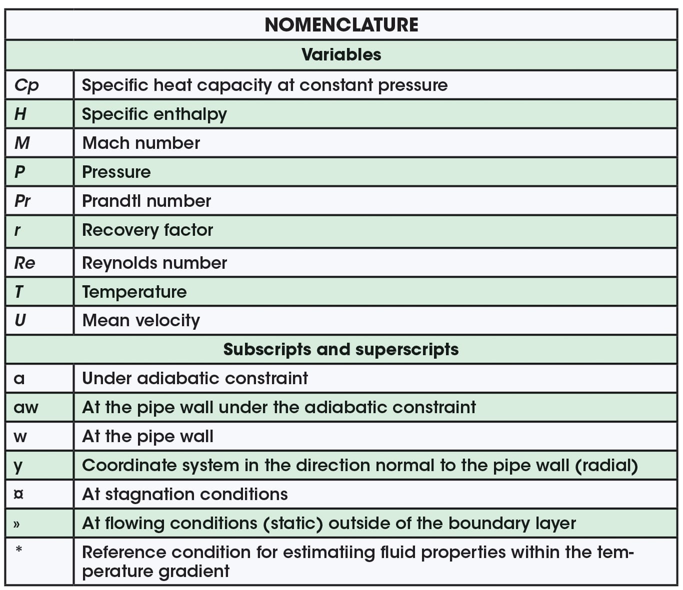
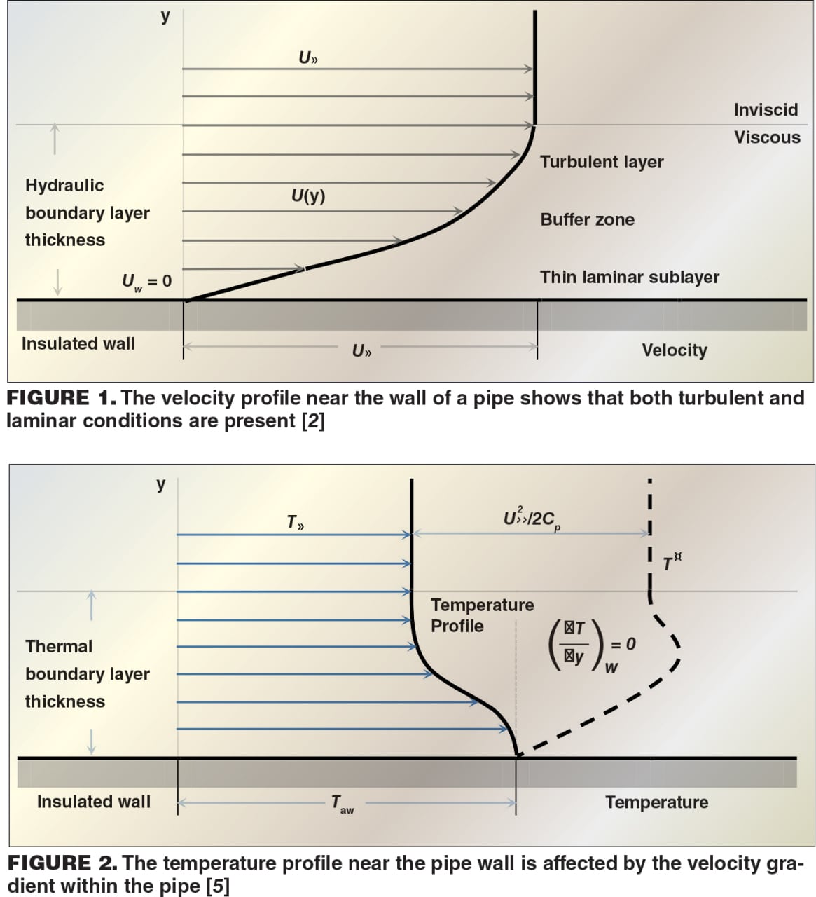
Before attempting reconciliation of the various notions related to wall temperatures, it is useful to recall Prandtl’s theory of the boundary layer, which envisions a small layer of fluid close to the pipe wall in which the viscous forces are significant due to the velocity gradient. However, outside of this layer, the core fluid flow approaches that of an inviscid fluid. The velocity gradient is established by the known boundary condition of zero velocity at the wall, as real fluids will “stick” to the pipe wall, and the maximum velocity is approached in the center of the pipe. For turbulent flow, this boundary layer consists of a laminar sublayer, a logarithmic outer layer and a buffer zone of some nominal thickness that transitions continuously between these sublayers [2]. The resultant velocity profile for a constant-area pipe in fully developed turbulent flow is shown in Figure 1. All variables, subscripts and superscripts presented in the equations and figures are defined in the Nomenclature section.
It is also useful to remember that the majority of resistances to flow within a pipe — the frictional losses themselves — are actually due to effects of this boundary layer, and that the friction factor is used as a means to determine these losses as a function of the mean velocity in the pipe. In addition, while a rigorous analysis of the energy and momentum balances that includes the boundary-layer effects would find that a slight modification of the terms would be required for turbulent flow (for instance, a momentum-correction factor of 1.018 for the logarithmic-law profile in turbulent flow), these correction factors are commonly ignored in engineering calculations. They tend to cancel out from mathematical expressions, and are minor when compared to the loss terms [2]. As a result, the typical energy and momentum balances as employed in engineering hydraulic calculations are still valid, even when recognizing the actual velocity profile.
For present purposes, we are concerned with the temperature profile that exists as a result of this actual velocity profile. However, before evaluating this, it is useful to also address heat-transfer considerations. For heat transfer within a pipe, a temperature gradient exists between the wall and the center of the pipe. In general heat-transfer calculations, it is convenient to define a bulk temperature. The bulk temperature is generally defined as the effective temperature across the gradient that drives the heat transfer with a wall of a given temperature. The normal calculations then proceed using this bulk temperature, and general experience is based on the most common heat-transfer situations — those that deal with phase transitions (in which case the effective temperature is essentially fixed at the saturation temperature) or liquid flow (in which case the effective temperature is taken as the average of the flowing temperatures). Heat transfer in gas flow is not as common, and when it does occur, the velocity is typically reduced. As a result, the accumulation of experience with heat-transfer design at petrochemical processing facilities does not typically include heat transfer with high-velocity gas streams.
Adiabatic wall temperature
An area of practice that does offer experience with this situation is aeronautical engineering. A summary of the cumulative theoretical and experimental work in this area, provided by Eckert [3, 4], indicates that for high-speed gas flow, the fluid temperature at the wall is significantly greater than the static (flowing) temperature. Also described in literature by Shapiro [5], is the phenomenon of the temperature profile of a gas in response to the actual velocity profile, where the steady-state temperature distribution shows an adiabatic wall temperature Taw being greater than the free-stream temperature T», yet less than the free-stream stagnation temperature, T¤. This temperature profile is shown in Figure 2.
The experimental work in this area has confirmed that the adiabatic wall (recovery) temperature approaches, but does not reach, the stagnation temperature. A recovery factor is thus defined as the amount of the stagnation temperature that is recovered as the fluid decelerates to zero velocity at the wall, based on the actual temperatures achieved [3]. Equation (1) shows an expression for the recovery factor, r.
![]() (1)
(1)
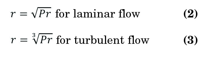
The subscripts aw, », and ¤ are for the adiabatic wall, static and stagnation temperatures, respectively. The recovery factor, r, has been found to be dependent on Pr, and for 0.5 < Pr < 5, the recovery factor is estimated as shown below in Equations (2) and (3) for laminar and turbulent flow, respectively [3].
A detailed analysis of the turbulent boundary layer, presented by Shapiro [5], finds that the adiabatic-wall recovery factor is a function of Pr and the ratio of velocities between the laminar sublayer and the edge of the boundary layer. While admittedly, this velocity ratio is not accurately known for compressible flow, it does indicate the boundaries for r when Pr < r < 1. Development of a more accurate expression for the recovery factor is further complicated by the difference in the hydraulic and thermal boundary-layer thicknesses. Nonetheless, Shapiro presents an analytical expression [5], which has been further developed by Tucker and Maslin [6], and shows that this expression approaches the expression for turbulent flow shown in Equation (2) at high Reynolds number values and Mach numbers less than one.
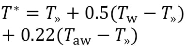
The computation of Pr requires the selection of a reference temperature, T*, at which to evaluate the fluid properties, and Eckert’s work states that the constant-property calculations could be used with a reference temperature defined as in Equation (4) below [3].
 (4)
(4)
For adiabatic flow, Tw is equivalent to Taw; therefore, the reference temperature is given by Equation (5).
![]() (5)
(5)
Further research at Mach numbers much greater than one found that an enthalpy approach (as opposed to the temperature approach) was needed. However, the present discussion is limited to flowing velocities having Mach numbers less than or equal to one.
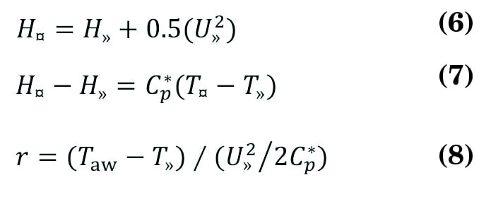
The difference between the stagnation and static temperatures can be expressed as a function of the velocity and the specific heat capacity at constant pressure (evaluated at the reference temperature [3]), based on the fluid specific enthalpy, as defined in Equations (6), (7) and (8).
The experimental and theoretical work outlined by Eckert [3, 4] is based on high-velocity gas flow relative to flat plates; nonetheless, additional work for the now-defunct National Advisory Committee for Aeronautics (NACA) [7,8] experimentally determined the recovered wall temperatures in adiabatic and diabatic airflow in pipes at a range of Reynolds and Mach numbers. Figure 3 is adapted from NACA Technical Note (TN) 4376 [8] and shows how the recovery factors vary with changing Reynolds number values.
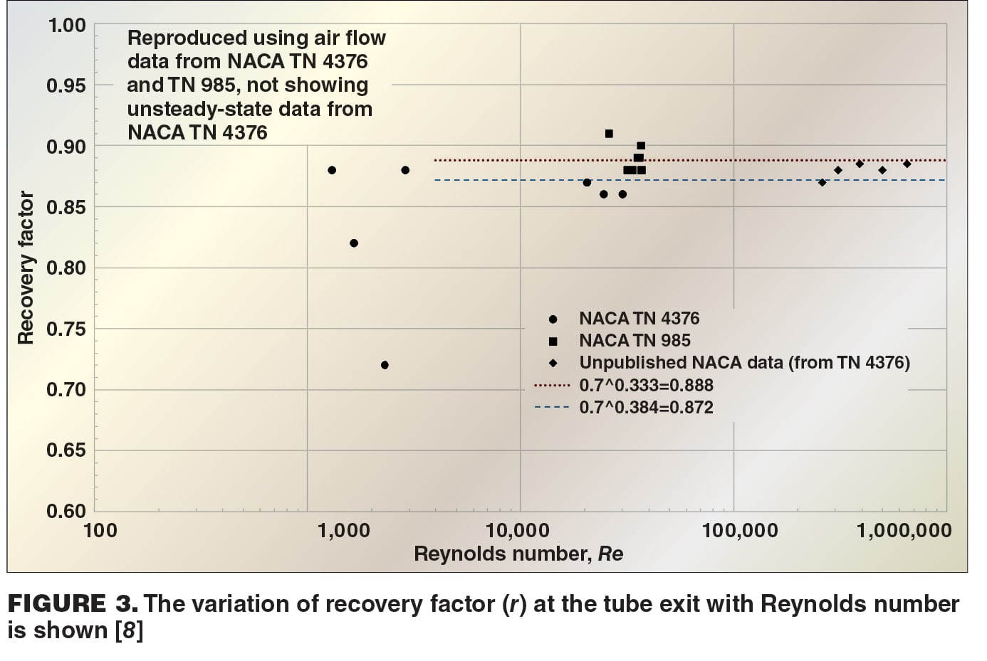
NACA Technical Note 4376 states that “In the turbulent flow region (Reynolds numbers above 3,000) the temperature recovery factor is nearly independent of Reynolds number. The average value is 0.88, which agrees with values for flow parallel to flat plates.” The experimental evidence for pipe flow was found to be in substantial agreement with the experimental evidence for flat plates.
The development of the adiabatic-wall-temperature recovery factor for turbulent flow to this point has been focused on flat plates or flow within pipes, and it is not obvious whether this analysis applies in situations involving a significant change in the fluid flowing direction, such as at an elbow or a tee. The velocity at the wall is still assumed to be zero, but the boundary layer is not developed in the same way as with flat plates at a given angle of attack or for pipes. Experimental work on the heat transfer for jets impinging on surfaces may provide some guidance in this evaluation, although much of the focus is on the effects on heat transfer when changing the distance or angle of attack between the jet source (nozzle, orifice or end of pipe) and the flat plate. In the jet-impingement studies found by the author, the discharge is directed at a flat plate having a large surface area, without restriction or redirection of the flow, so it is not directly applicable to configurations like a tee in pipe flow — nonetheless, some temperature recovery occurs. Per work by Goldstein and others [9], the recovery factor for the impingement of air on a surface is independent of the jet Reynolds number, but is dependent on the jet to impingement plate spacing. In this work, a minimum recovery factor of 0.7 was determined, which is the approximate value of Pr for air.
It would appear that the prudent course of action would be to use the bounds of the recovery factor depending on the goals of the analysis. For the case of the determination of the adiabatic wall temperature for use in the low-temperature estimate for material specification, the lower bound of the recovery factor would provide this estimate, as shown in Equation (9).
![]() for lowest recovery (9)
for lowest recovery (9)
In addition, in the evaluation and development of the adiabatic-wall-temperature recovery factor, only noncondensable gases have been considered. It is conceivable that a vapor stream may experience flowing temperatures below its dewpoint, thus possibly condensing within the core stream. It is possible that at the wall, the shearing work and frictional heating is sufficiently high to ensure that there are no liquid droplets touching the wall, and the flow behaves as an annular two-phase flow that can be treated as a gas for practical purposes. On the other hand, it is possible that the condensed liquid droplets can contact the wall, which may result in additional cooling at the wall as the liquid is vaporized. The evaluation of the adiabatic wall temperature for high-speed condensable vapor flow remains as further work.
Application and examples
One of the direct applications of this information would be the screening of potential low-temperature issues caused by low-flowing temperatures in all-gas flow systems. The recovery factor for these cases can be determined as a function of Pr at the reference temperature T* as described by Eckert [3, 4], or perhaps in the more detailed analysis of Shapiro [5]. This recovery factor can then be used to determine an actual adiabatic wall temperature. The recovery temperature should then be compared to the minimum design metal temperature (MDMT) of the piping system for identification of potential low-temperature cases. In addition, any analysis that is being performed involving heat transfer between the fluid and the pipe should be based on the effective temperature differential between the pipe wall temperature and this adiabatic wall temperature.
A practical application of the adiabatic wall temperature evaluation can be found in natural-gas processing facilities, where discharges from pressure-relief or depressurization valves may involve high-velocity noncondensable gas. Evaluations of discharge piping that are performed assuming adiabatic flow yield flowing temperatures and velocities. These flowing conditions can be used to determine the stagnation enthalpy, and thus the stagnation temperature, which can then be used in the calculation of r.
Calculation example
As an example of wall-temperature determination, consider the flow of 25,000 lb/h of methane at 400 ft/s within an 8-in. Schedule 40 pipe having a stream temperature of –20°F. The following steps were performed, using the equations defined previously in this article, as well as the properties of methane obtained from the National Institute for Standards and Technology’s (NIST) standard reference data program, Refprop v. 9.0 [10]:
- Use the velocity and flowing enthalpy to determine the stagnation enthalpy per Equation (6)
- Perform an enthalpy-entropy flash at the stagnation enthalpy and flowing entropy to obtain the stagnation temperature
- Iterate on the reference temperature to obtain the specific heat capacity at constant pressure, viscosity and conductivity for use in determining Pr
- The stagnation temperature is used as the adiabatic wall temperature for the first step in the iteration in this example, but a better estimate can be determined using an estimated recovery factor of 0.88 and Equation (8)
- The reference temperature is calculated based on Equation (5) at each step
- The fluid properties are re-evaluated at the reference temperature and the flowing entropy, and Pr is
recalculated - Calculate r based on Equations (2), (3) or (9). Equation (3) was used in this
particular example - Calculate an adiabatic wall temperature based on Equation (1)
- Iteration is continued until the solution converges on an adiabatic wall temperature
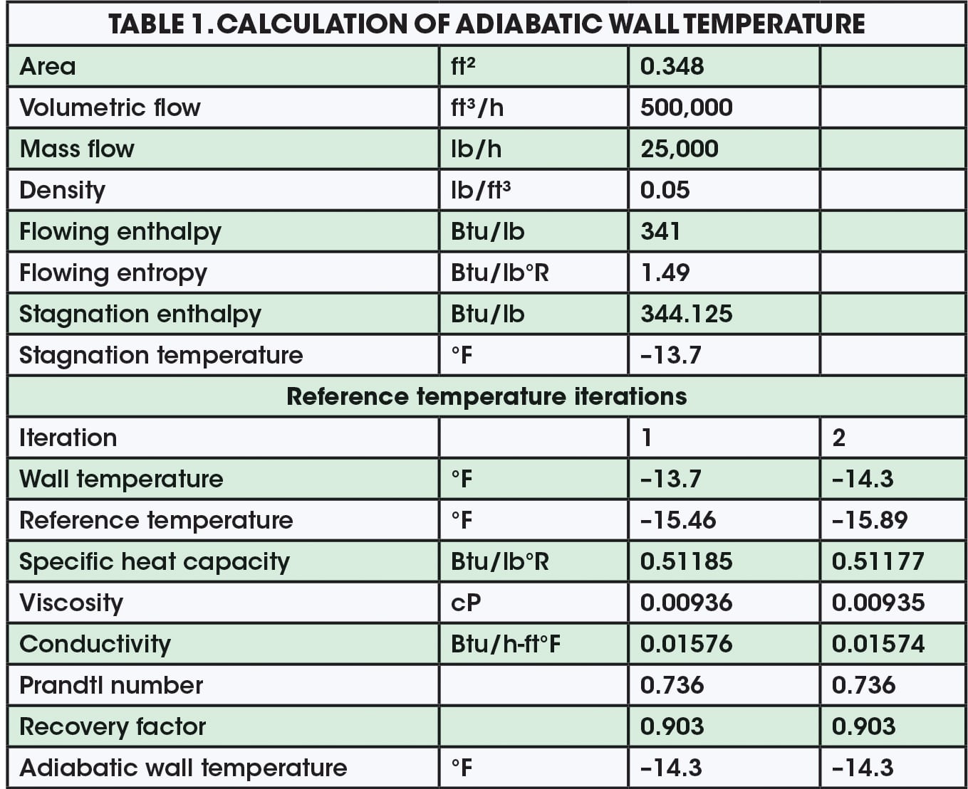
In this case, an adiabatic wall temperature of –14.3°F is calculated. Table 1 gives a summary of the parameters used in this example for the iterative determination of the adiabatic wall temperature. One will find that by using an estimated recovery factor of 0.88 to generate the reference temperature from Equation (8), iteration is generally not needed, as Pr does not vary significantly over the temperature range.
Design chart for methane
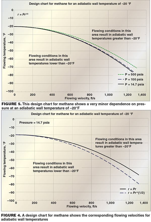
Alternatively, design charts can be prepared for a specific gas and material specification to speed the screening of potential low temperatures. Using the fluid properties of methane, obtained by means of the NIST Refprop program [10], the locus of flow conditions that would result in an adiabatic wall temperature of –20°F were identified for the Eckert estimate for turbulent pipe flow using Equation (3), as well as the low temperature estimate using Equation (9), with the reference temperature evaluated using Equation (5). As shown in Figure 4, flow conditions above the line result in adiabatic wall temperatures greater than –20°F, while conditions below the line result in adiabatic wall temperatures less than –20°F.
The properties of methane in the regions investigated are primarily dependent on temperature; however, there is some pressure dependence. The design chart as described above is generated for other static (flowing) pressures, using the turbulent recovery factor of Equation (3), and is shown in Figure 5. One will note the minor effects of pressure on the design charts. Design charts, along with the correlations described in this article, are effective ways of determining adiabatic wall temperature in high-velocity gases.
Edited by Mary Page Bailey
Acknowledgment
The author would like to thank Georges A. Melhem and Dale L. Embry for their review of the content of this manuscript.
References
1. Shackelford, A.E. and Pack, B.A., Overpressure Protection: Consider Low Temperature Effects in Design, Chem. Eng., July 2012, pp. 45–48.
2. Benedict, R.P., “Fundamentals of Pipe Flow,” John Wiley & Sons, Inc., New York, 1980.
3. Eckert, E.R.G., Survey on Heat Transfer at High Speeds, Aeronautical Research Laboratory (ARL) Technical Report 189, Dec. 1961.
4. Eckert, E.R.G., Survey of Boundary Layer Heat Transfer at High Velocities and High Temperatures, Wright Air Development Center Technical Report 59–624, April 1960.
5. Shapiro, A.H., “The Dynamics and Thermodynamics of Compressible Fluid Flow,” Ronald Press Co., N.Y., 1953.
6. Tucker, M. and Maslin, S.H., Turbulent Boundary-Layer Temperature Recovery Factors in Two-Dimensional Supersonic Flow, NACA Technical Note No. 2296, 1951.
7. McAdams, W.H., Nicolai, L.A. and Keenan, J.H., Measurements of Recovery Factors and Coefficients of Heat Transfer in a Tube for Subsonic Flow of Air, NACA Technical Note No. 985, June 1945.
8. Deissler, R.G., Weiland, W.F. and Lowdermilk, W.H., Analytical and Experimental Investigation of Temperature Recovery Factors for Fully Developed Flow of Air in a Tube, NACA Technical Note No. 4376, Sept. 1958.
9. Goldstein, R.J., Behbahani, A.I. and Heppelmann, K.K., Streamwise Distribution of the Recovery Factor and the Local Heat transfer coefficient to an Impinging Circular Air Jet, International Journal of Heat and Mass Transfer, Vol. 29(8), 1986, pp. 1,227–1,235.
10. Lemmon, E.W., Huber, M.L. and McLinden, M.O., NIST Standard Reference Database 23: Reference Fluid Thermodynamic and Transport Properties-REFPROP, Version 9.0, National Institute of Standards and Technology, Standard Reference Data Program, Gaithersburg, Md., 2010.
Author
 Aubry Shackelford is president and principal engineer at Inglenook Engineering, Inc. (15306 Amesbury Lane, Sugar Land, TX 77478; Phone: 713-805-8277; Email: [email protected]). He has over ten years of experience in process safety management in general, with particular emphasis on pressure-relief design. Shackelford has also helped author several guidelines related to pressure relief for the American Petroleum Institute (API), the International Organization for Standardization (ISO) and the Center for Chemical Process Safety (CCPS). He has a B.S.Ch.E. from Northeastern University and holds affiliations with AIChE, NSPE and SPE.