Utilizing ‘Tolerance Intervals’ can help to set more realistic specification ranges, especially when only small amounts of data are available
Specifications provide a framework by which one can gage whether products have been manufactured successfully. They identify a product’s key characteristics and, for each attribute, quantify how much deviation from a target value is allowed. Normally, specification ranges are derived from either the “voice of the customer” (that is, customer requirements) or the “voice of the process” (that is, process capabilities).
For example, when formulating a material that will be sold in tubes, what rheology or flow properties should the product have? Customers ideally want the substance inside the tubes to be stiff enough (with a high enough yield point) so that it won’t flow unintentionally, but thin enough that when a reasonable amount of force is applied, the product dispenses. To control this, a viscosity specification would be created to guide manufacturing.
In both cases, whether specifications are dictated by customer or process requirements, development engineers must carry out enough experimentation to uncover how much the product and its properties are affected by innate manufacturing variability. In addition, when specifications are driven by customer needs, one must substantiate that the manufacturing process is capable of unfailingly supplying product that meets those obligations; if the process cannot meet them, then it should be modified until it can.
After collecting pre-production data, how should that information be employed to predict future product variability? The chemical process industries (CPI) currently have no widely accepted, standard way of establishing process capability-based specification limits. Some companies take minimum and maximum values observed during product development and scale-up and then utilize them as specification boundaries. Others rely on statistical concepts, such as the widely known Six Sigma method, to establish acceptance criteria.
When pre-production measurements or test results originate from normally distributed populations — a very common situation — the equations below stipulate the Six Sigma outer limits. They depend on the data’s mean,µ, and standard deviation, σ:
Lower release limit ( LRL) =µ – 3 σ
Upper release limit ( URL) =µ + 3 σ
( Note: Six Sigma represents the span of –3 to 3 standard deviations. For large amounts of data, that span covers 99.73% of all measurements if the data are normally distributed.)
What many don’t realize is that both specification-setting methods mentioned above are only appropriate when appraising large data sets (containing at least 30, but maybe 50 or more data points). They are invalid when just a few data points have been acquired. However, many companies these days have a conflicting mandate — to shorten product-development schedules so products can be delivered faster to the marketplace. This frequently translates into less time available for experimentation in the laboratory or in pilot plants (and thus, less data generated during preproduction).
When creating specification ranges from a limited number of data points, boundaries generally end up being too close together because small “sample” quantities seldom exhibit the degree of variation found in larger data sets. With undersized or inadequate specification ranges, some future output will be flagged as being out of specification (OOS), when in reality, nothing is wrong with it; the OOS test result or measurement emerged from normal process variation — not some aberration of the manufacturing process.
The Tolerance Intervals method
To balance a company’s competing objectives (to be “first to market” versus ensuring outstanding product quality), more businesses should adopt Tolerance Intervals (TIs) as a specification-setting technique. This method compensates for pared-down data sets, and produces wider, more realistic specification ranges while requiring just a fraction of the customary amount of pre-production data. TIs are defined by:
- The number of data pointsobtained
- The minimum proportion of a population that must be covered by the TI (50, 75, 90, 95 or 99% are typical values picked)
- The confidence level chosen (90, 95 or 99% are common values), indicating the likelihood that the range or interval will cover the proportion of a population selected
TI endpoint equations [ 1] are expressed similarly to the Six Sigma method, with k 2, the tolerance factor for normal, two-sided population distributions, replacing the three values in the earlier definition of LRL and URL:
LRL =µ – k 2 σ
URL =µ + k 2 σ
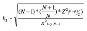
The equation shown below furnishes an approximate value for k 2, where:
N = the number of data points
z = the critical value of a standard normal probability
σ = the minimum proportion of a population, %
σ = a confidence level, %
σ 2 = a Chi-Square distribution
x 2 1– ρ , N –1 = Lower tail critical value of Chi-Square distribution
z ((1– ρ )/2) =Critical value of the standard normal distribution for a cumulative probability of ((1 – σ)/2)
A practical example
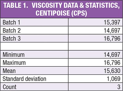
Recently the author’s company developed a new product whose viscosities are very similar to those of another product that has been produced for a while. Three pilot plant batches were made, with the viscosity data and resulting statistics shown in Table 1.
What proportion of a population and confidence level should be chosen when creating the TI specification ranges for this new product? Through some evaluation, the author found that selecting a 99% proportion of a population and a 90% confidence level usually works well, creating specification ranges that are neither too wide nor too narrow.
Where:
N = Number of data points = 3
ρ = Proportion of population to be covered = 99%
z ((1– ρ )/2)) = The critical value of a standard normal probability = z ((1–0.99)/2) = z 0.005 = –2.58
z 2 ((1– ρ )/2)) = (-2.58) 2 = 6.65
ρ = Confidence Level = 90%
x 2 1– ρ , N –1 = Lower tail critical value of Chi-Square distribution = x 2 0.1,2 =0.211
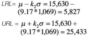
k 2 = [2*(4/3)*.6.65/0.211] 0.5 = 9.17
Thus:
Table 2 summarizes the specification ranges created by the three specification methodologies (Minimum/Maximum, Six Sigma and TIs) discussed here. Clearly, the Tolerance Interval release limits are significantly wider than those generated by the other two approaches.
As mentioned previously, the new product’s viscosities are very similar to those of another product that’s been manufactured for a while. Table 3 contains statistics for the established product. Comparing the proposed specification ranges in Table 2 with information acquired from the older product is informative. Assuming both products have identical viscosity-population distributions allows one to estimate OOS frequencies for the three specification ranges (shown in Table 4). This demonstrates how unsuitable the first two methods can be at creating specification ranges for situations involving small data sets.
It should be noted that the OOS percentages listed in Table 4 are for a single quality parameter. If an invalid methodology is used to create the specification limits of more than one quality parameter, the likelihood of making OOS product increases correspondingly. This is illustrated by the two-factor probability equation shown below:
P( A or B) = P( A) + P( B) – P( A and B)
If the odds of having OOS product by parameter A are 10%, or by parameter B are 10%, then the odds of having OOS product from either A or B are calculated using the following equation:
P( A or B) = P( A) + P( B) – P( A and B)= (1/10)+(1/10) – [(1/10)*(1/10)] = 19%
Considering the negative consequences typically associated with manufacturing OOS products, they should be avoided, especially when they arise from routine variation, not from a process deviation that could adversely impact a product’s quality.
Admittedly, small data sets sometimes contain considerable variability. Applying the Tolerance Interval method to such data can lead to very wide specification limits that are neither feasible nor desirable. For instance, the lower viscosity-release limit could end up as a negative number, which is physically impossible. In all instances, before calculating a TI, the following should be done:
Check for and exclude outliers/anomalies from the data set. Several statistical methods are available for detecting outliers.
If the calculated TI is still wider than expected or desired, proceed with one of the following options:
Option 1. Propose a narrower, more pragmatic specification range and identify what confidence level corresponds with it.The confidence level associated with a tighter, but more reasonable, specification range can be computed. If the confidence level turns out to be sufficiently high, the adjusted specification range should be adopted. An example of how to do this is discussed below. Option 2. Generate some supplementary preproduction data.Producing just a few additional test results (not the 30–50 data points required by other specification setting techniques) ordinarily leads to enough convergence between observations so that the Tolerance Interval will shrink considerably. The k 2 value is driven down through increased knowledge about the new product, and the standard deviation generally decreases as well. This is demonstrated in an example below.
Calculating confidence level
Discussed next are recommendations for calculating the confidence level of a designated specificaiton range. Table 5 shows viscosity data associated with a very thick product. Since these data were not consistent, the proposed viscosity range using Tolerance Intervals, as shown in the middle column of Table 6, was quite wide. The LRL (at a 90% confidence level) was unacceptably low at only 23,306 cps. As a result, an alternative viscosity range of 200,000–500,000 cps was proposed and evaluated. What confidence level coincides with that range when 99% of future production viscosities must fall within that range?
Referring to Figure 1, since the average viscosity of 384,333 is not the midpoint of the proposed range of 200,000 – 500,000, both sides of the population distribution will be examined separately. For the lower tail of the distribution:
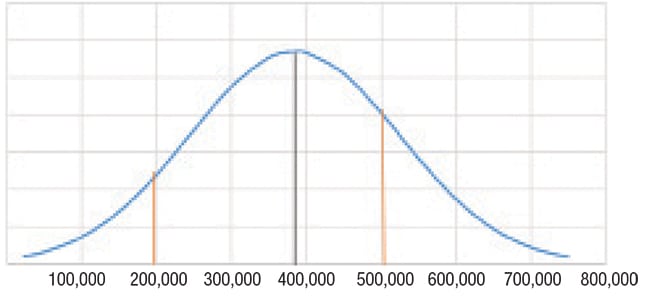
Figure 1. Shown here is the predicted population distribution for the calculating confidence level example
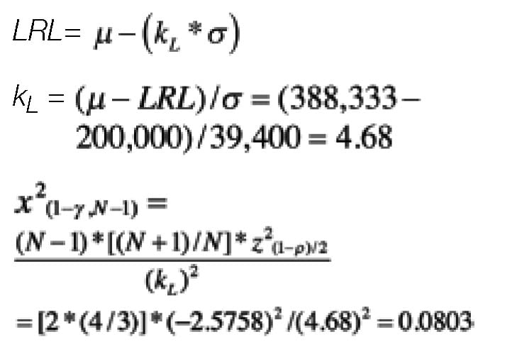
To determine 1–γ one should specify the degrees of freedom ( N–1) and calculate the Chi-square cumulative distribution function (Some spreadsheet programs or online calculators can do this computation). The result is 0.332. The confidence level for the lower portion of the specification range is:
γ = 1 – 0.332 = 66.8%
This means there is a 66.8% confidence level that future test results will be > 200,000 cps.
Performing similar calculations on the upper portion of the prospective specification range reveals that there is only a 35.8% confidence level that prospective viscosities will be < 500,000 cps.
In situations like this, where the confidence level is not very high, a risk assessment should be carried out. Is there a high likelihood that OOS results will occur down the road? If the risk of generating OOS results is unacceptably high, select one of the options below:
Reducing Tolerance Intervals
Providing supplementary information can help to reduce TIs. With over-the-counter drugs, the LRL and URL for active ingredients are typically set at or within 10% of the target level. Table 7 provides an example of a situation that involved augmenting the initial test data. As shown, the row with the sought-after release limits is highlighted. Below that, Tolerance Intervals were calculated using test results from only three pilot batches. All TIs were wider than the targeted release limits — not desired.
The effect of supplementing the original data with test results from three additional pilot batches is shown on the bottom row of Table 7. Each TI contracted considerably, with all TIs now falling inside the prescribed boundaries. This demonstrates how supplying just a few extra data points can have a pronounced impact on a TI because statistical uncertainty is reduced.
References
1. NIST/SEMATECH e-Handbook of Statistical Methods, http://www.itl.nist.gov/div898/handbook/prc/section2/prc263.htm, May 23, 2016.
Author
 Noel L. Sutton is a senior principal process development engineer at Amway (7575 Fulton E., Ada, MI 49355; Phone: 616-787-5714; Email: noel_sutton@amway.com). In this capacity, he has scaled up processes for a wide variety of products. He began his career as a process design engineer at Amway for four years, then gained over 32 years experience in process development at both Helene Curtis, Inc. and Amway. Sutton holds a B.S.Ch.E. from the University of Washington, and a Master’s in engineering management from Northwestern University. He is a member of AIChE.
