The recommended velocities for fluids’ transportation must be updated periodically to obtain the optimum value of the pipe diameter in the current economic conditions
To arrive at the optimum diameters for pipes, the heuristic criteria of recommended velocity has been used in the past. However, the values used as criteria are not updated frequently, despite changes and fluctuations in the economy. Because the recommended velocities are likely out of date, the resulting pipe diameter values can be far from reality.
In the article “Updating the rules for pipe sizing” [1], an update of the recommended velocity was presented, based on the energy costs from 2008. This analysis showed that the recommended velocities are highly sensitive to energy and material costs. In this article, the recommended velocities have been updated based on 2017 prices for energy and current prices for highly used materials in the industry.
Optimizing the pipe diameter
Given the uncertainty of fossil fuel depletion and the volatility in its prices, there is a growing general necessity to optimize processes in an effort to locate economic alternatives where operating and investment costs converge to a minimum that increases efficiency. One way to reduce costs in process plants is to optimize the variables that affect the transport of fluids. For example, pumping systems (pumps, motors, pipes and fittings) represent a high operational cost; they account for between 25 and 50% of energy use in certain plant operations. This cost is directly related to the diameter of the pipe.
As presented below, the optimization of pipe diameters can be accomplished using equations that relate the recommended velocity of fluids and the cost of energy.
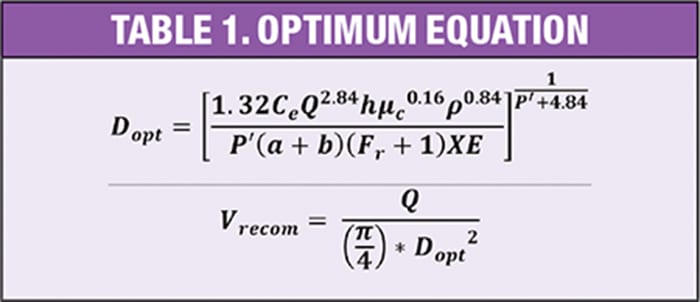
To determine the recommended velocities and compare what was published 10 years ago [1] to 2017, Equation (1) is used (Table 1, top). It is presented in Ref. 2. For the calculation of the recommended velocities, Equation (2) is used (Table 1, bottom). As shown in Equations (1) and (2) and Table 1, velocities are intrinsically related to the properties of the fluid and a series of economic parameters, including energy costs, pipe materials and other operational criteria. All variables are given in Table 2.
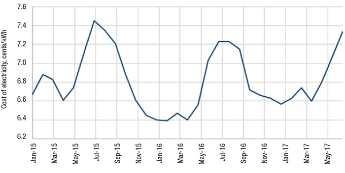
Figure 1. The graphs shows the average cost of electricity for the U.S. for 2015–2017
U.S. energy cost variation
Because the determination of optimum diameter is strongly related to the cost of energy, Figure 1 shows the variations in the cost of electricity for the industrial sector in the last two years and Table 3 shows the average cost of electricity in recent months [3]. Figure 1 indicates that the price of electric power in the U.S. has remained technically constant, with a maximum variation of 10.0% compared to the average. To obtain the cost of electric power (Ce) needed for Equation (1), the cost of electric power for the U.S. industrial sector was averaged from January to July 2017. That information is shown in Table 2.
Table 4 shows the values of the parameters to be used in Equation (1). In addition, values of parameters X and P were obtained for six of the most commonly used materials in the chemical and petrochemical industries. The costs of these materials were obtained from international suppliers and were analyzed in particular. The materials analyzed are listed below:
- Aluminum schedule-40
- Brass schedule-40
- Carbon steel A106 grade B, schedule-80
- Carbon steel A53 grade B, schedule-STD
- Copper-nickel class 200
- Stainless steel A312 Grade 304L, schedule-40S.
Table 5 shows the values of X and P by the type of material analyzed. These were obtained from pipe quotes found on Internet sources and from Producer Price Indexes (PPI) [4].

Calculation protocol
The behavior of the recommended velocities was compared using the density and viscosity at different temperatures, for each of the materials, keeping the pressure constant at 19.10 psia. The fluid used for the calculation was water.
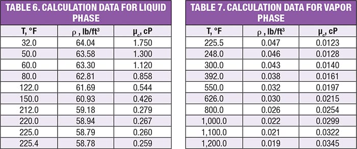
Table 6 shows the values used in the calculations for the liquid phase.For each temperature mentioned in Table 5, the recommended velocities in the liquid phase were obtained for different densities (Figure 2) and different viscosities (Figure 3) for each material. Table 7 shows the values used for the calculation for the liquid phase. And for each temperature mentioned in Table 6, the recommended velocities in the vapor phase were obtained, also with varying density (Figure 4) and viscosity (Figure 5), for each material.
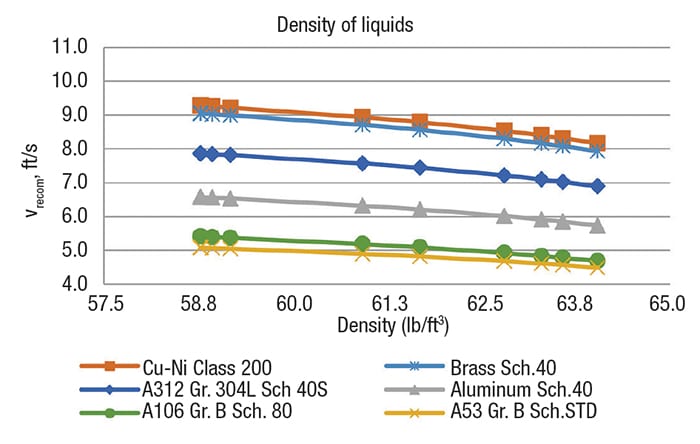
Figure 2. The graph shows the recommended velocity versus density of liquids
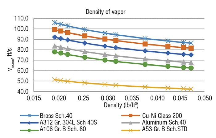
Figure 3. The graph shows recommended velocity versus density of vapors
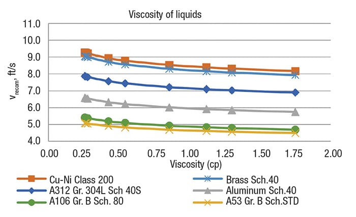
Figure 4. The graph shows recommended velocity versus viscosity of liquids
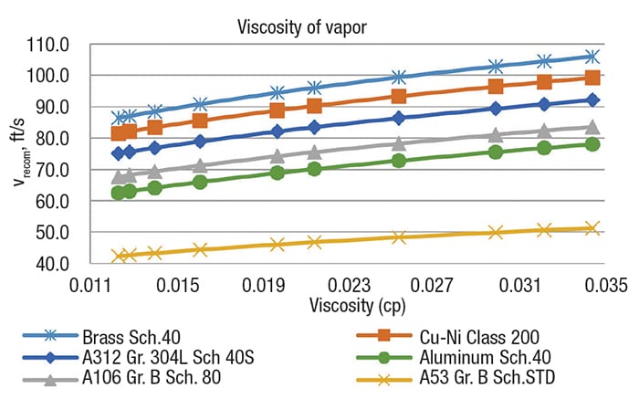
Figure 5. The graph shows recommended velocity versus viscosity of vapors
The order of recommended velocities, from greatest to least, is the following for both phases (liquid and vapor): Brass schedule-40 and copper-nickel class 200 > Stainless steel A312 grade 304L, Schedule-40S > Carbon steel A106 grade B, schedule-80 > Aluminum schedule-40 > Carbon steel A53 grade B, schedule-STD.
The order above indicates that the most expensive materials will have the highest recommended velocities and the smallest diameters, and vice versa. However, it is important that, with regard to the service being handled, the most appropriate material is selected.
Analyzing changes in velocities
To compare the data obtained here with the costs over the last ten years, four materials were selected and analyzed in both cases:
- Aluminum schedule-40
- Brass schedule-40
- Carbon steel A53 grade B, schedule-STD
- Stainless steel A312 grade 304L, schedule-40S
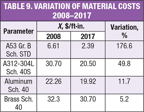
Table 8 shows the influence of the change in energy and material costs over the last ten years, and Table 9 shows the comparison between the costs of materials over the same time period.
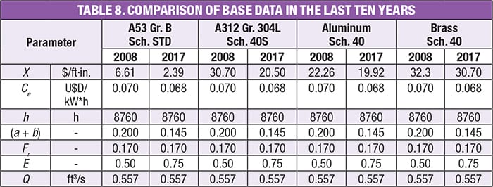
The results of the comparative analysis of recommended velocities show that, although the costs of energy (3.24% in the last ten years) and the materials studied have decreased (Table 9), the recommended velocities have increased, making the optimum diameters of the pipes decrease by up to 35.0% compared to 2008.
The above result is due mainly to two factors. Required efficiency of pumps and motors increased from 50 to 75%. This is because at present, the design of pumping equipment follows the requirements established in standards such as American Petroleum Institute standard 610, which indicates that operation must be as close as possible to the best efficiency point (BEP), which is the flow at which the pump system is operating its highest efficiency.
Depreciation and maintenance factors have decreased because more control exists over maintenance procedures and standards, so plants can operate for longer times.
Example calculation 1
For this example, the following information and values are used:
- The pipe material is carbon steel A53 grade B, schedule-STD
- Fluid is water at 60°F
- Flow (Q): 1.625 ft3/s
- Density (ρ): 50.0 lb/ft3
Using this information, a recommended velocity (vrecom) of 4.95 ft/s is obtained, as shown in Figure 6. The cross-section area for these conditions is the following:
S= Q ⁄ vrecom= 1.625 ⁄ 4.95 = 0.3285 ft2
This cross-section is reasonably close to that of a 8-in. dia. pipe for this material ( S = 0.3474 ft2). Comparing the recommended velocity value that would be obtained with the same data ten years ago (4.38 ft/s), it is observed that the recommended velocity increased by 13.0% and with it, the area of the cross-section increases:
S = Q ⁄ v recom= 1.625 ⁄ 4.38 = 0.3710 ft2
Since this value is higher, it is necessary that the tube diameter is 10-in. dia. (S = 0.5475 ft2) to achieve the required value.
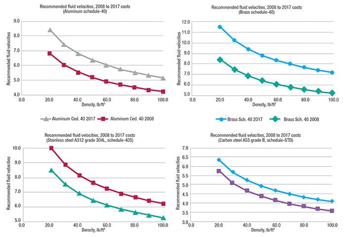
Figure 6. Recommended fluid velocities, 2008–2017 are plotted here
Example calculation 2
For this example, the following information and values are used:
- Pipe material: Stainless steel A312 Grade 304L, Schedule-40S
- Fluid: water at 60°F
- Flow (Q): 1.625 ft3/s
- Density (ρ): 30.0 lb/ft3
Using this information, a recommended velocity (vrecom) of 8.88 ft/s is obtained, as shown in Figure 6. The cross-section area for these conditions is the following:
S = Q ⁄ vrecom= 1.625 ⁄ 8.88 = 0.1830 ft2
This cross-section is reasonably close to that of a 6-in. dia. for this material ( S = 0. 2006 ft2). Comparing the recommended velocity value that would be obtained with the same data ten years ago (7.50 ft/s), it is observed that the recommended velocity increased by 18.0% and with it, the area of the cross-section increases:
S = Q ⁄ vrecom= 1.625 ⁄ 7.50 = 0.2166 ft2
As in the first example, the value of the section is greater, so it is necessary that the diameter of the tube is 8-in. dia. (S = 0.3474 ft2) to achieve the required value.
Concluding remarks
Revised values for the recommended fluid velocities in this article have proved to be highly sensitive to energy and material costs. However, there are two main factors related to the increase in recommended fluid velocities and the decrease in optimal diameters: increase in the required efficiency of pumping equipment and decrease in the depreciation and maintenance factors. It is important to remember that these factors have changed due to the application of stricter standards, focused on the efficient use of resources. In general terms, recommended fluid velocities have increased up to 35% due to the decrease in the cost of materials since 2008.
The analysis serves as a guide for the management of fluids at different conditions, while maintaining the integrity of the pipes. So it is important to continue updating the recommended fluid velocities to consider fluctuations in energy and material costs used at least every five years, and maintain an optimal design.
Edited by Scott Jenkins
References
1. A. Anaya Durand, Anaya A. and others, Updating the rules for pipe sizing, Chem. Eng., vol. 117, no. 1, p. 48, 2010.
2. Skelland, A.H.P., “Non-Newtonian flow and heat transfer,” Wiley. New York, 1967.
3. U.S. Energy Information Administration. Electric Power Monthly: www.eia.gov/electricity
4. U.S. Bureau of Labor Statistics, 2017. www.bls.gov.
5. Kern, Donald Q., “Process Heat Transfer.” Edit. Continental. México, 1999.
6. Branan, Carl R., “Rules of thumb for chemical engineers.” Gulf Professional Publishing. 2002.
6. Crane Corp., “Flow of Fluids Through Valves, Fittings and Pipe.” Technical Paper No. 410. 2009.
7. ANSI/API Standard 610. “Centrifugal pumps for petroleum, petrochemical and natural gas industries” 11th ed., September 2010.
9. McMaster-Carr, 2017. www.mcmaster.com
Authors
 Alejandro Anaya Durand (Parque España No. 15b Col. Condesa, C.P. 06140, Mexico; Email: [email protected]) is a professor of chemical engineering at the National University of Mexico (UNAM), and has over 55 years experience in project and process engineering. He retired from Instituto Mexicano del Petroleo (IMP) in 1998 after holding top positions. For 50 years he has been an educator in chemical engineering in several universities in Mexico, and presently he is also a consultant at several engineering companies. He has published over 250 papers related to engineering and education; is a Fellow of the AIChE; a member of National Academy of Engineering; and has received the main chemical engineering awards Mexico. He holds a M.S. in project engineering from UNAM.
 Jesús Antonio Soto Estrada (Rosa Amarilla #149-7, Col. Molino de Rosas, C.P. 01470, Álvaro Obregón, Mexico City, México; Phone: +52 (55) 55 3513 0521; E-mail: [email protected]) is a chemical engineer with five years of work experience on projects in the chemical and petrochemical sectors in the areas of processes and quality management, and is a chemical engineering master’s student in process engineering at UNAM.
 Nayeli Cabrera Delgado (Granjas Ave. #617, Mexico City, Azcapotzalco, Mexico 02519; Phone: +52 55 61 11 92 64; Email: [email protected]) is a chemical engineer with seven years of work experience in the petroleum and environmental sector, taking part of different relevant projects for diverse Mexican institutions in the areas of process, quality and management. She is a third-semester master´s degree student in chemical engineering in the area of process engineering at UNAM. She had taken relevant courses related to the environment and oil sector at UNAM and Complutense University of Madrid. She led an engineering work team to finish a project to revamp two hydrodesulfurization units. She is an active member of Mexican Institute of Chemical Engineers (IMIQ).