The average large project in the chemical process industries (CPI) overruns its sanctioned budget, including contingency, by 21%. Even more alarming, 10% of large projects overrun their budget by more than 70%. These are findings based on research by the author and others. However, research also tells us that small projects, such as those managed at the plant level or those with little individual impact on company profit, tend to underrun their sanctioned amount, often significantly. This raises many questions regarding the techniques used to improve estimates of the contingency required in these situations.
The wide accuracy range of CPI projects indicates that there is tremendous uncertainty for owner capital projects of all sizes — much more than accepted rules-of-thumb may indicate (for instance, assuming that ±10% is considered “typical”). The overruns for large projects indicate that owners do not understand the risks and are not managing them well, or are biased to underfunding the risk because proper contingency might kill the project. Conversely, small project systems understand that there is variability in project costs, but find that the most expeditious way to keep moving forward is to have a cushion in each project budget to avoid “imperial entanglements” (punitive reaction to overruns).
Because each project is unique, it is often hard for an engineer or project leader to understand appropriate costs and to see cost biases (often their own) at work. Therefore, to improve the pricing of risks in their estimates and budgets, owners must address both technical and behavioral (bias) components of risk analysis and contingency estimating. Engineers responsible for estimating budgets or managing projects must sharpen their knowledge of risk and its quantification. The first step is to fully understand the concepts of risk, contingency and accuracy as applied to cost-estimation principles.
Risk, contingency and accuracy
For projects, risk is synonymous with uncertainty. International Organization for Standardization (ISO; Geneva, Switzerland; www.iso.org), Project Management Institute (PMI; Newton Square, Pa.; www.pmi.org) and Association for the Advancement of Cost Engineering (AACE) International (Morgantown, W.Va.; www.aacei.org) standards agree that anything (threats or opportunities) that might cause project outcomes to differ from plan is considered to be a risk. Contingency and reserves are how risks are funded in project budgets. Escalation and currency exchange are additional ways, but are outside the scope of this article.
A cost estimate includes two main parts: the “base” (essentially the risk-free costs other than specific allowances) and the “risks” (contingency, reserves, escalation and currency). Separate risk types are necessary, because there are different best practices for estimating and managing them. However, engineers should keep in mind that these risk types are not always easy to parse cleanly.
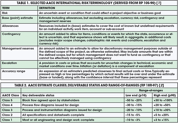
Accuracy, for cost-estimation purposes, is a shorthand term to describe estimates as predictions of uncertain outcomes — the estimate is a range of possible costs, not a discrete “number.” In that sense, a good estimator is one who knows, and is honest about, what he or she does not know. The person preparing the estimate must communicate the risks, the range of possible outcomes and, most importantly, how those two go together. Accuracy ranges are expressed as low and high percentages that bound the expectation of how final actual costs will differ from the estimate. For example, a range of +30%/–10% tells management that the final costs may be as much as 30% more or 10% less than the estimate after taking into account all of the identified risks. For a range statement to be complete, one must also state the confidence in this range; for instance, stating that 80% of the time, the project will be within these bounds. Also important to specify is the reference point that the range is based upon — it can be relative to the base estimate or to the funded amount, including contingency. Table 1 shows AACE International’s definitions from Recommended Practice (RP) 10S-90 [1] of these and other key risk terms.
Understand cost risk reality
Engineers need to know that there are no “standard” estimate ranges. AACE International’s RP 18R-97 (18R) [2] specifically states that an accuracy range must be “determined through risk analysis,” because every project’s risk profile is unique. RP 18R is designed to support owner phase-gate scope definition and decision-making processes by defining “classes” of estimates that align with typical industry phasing. It provides a “range-of-ranges” for estimate accuracy based on different levels of scope definition, as shown in Table 2. AACE’s message regarding cost risk is that we know in relative terms that estimate accuracy will improve as scope is better defined, but in absolute terms we can’t say by how much without risk analysis; risks vary too much between projects. Further, RP 18R states that its range-of-ranges excludes “extreme” risks. It also assumes that realistic, risk-based, unbiased contingency has been applied. Therefore, RP 18R’s ranges bracket the estimated amount including contingency. Unfortunately, many misquote AACE as providing specific ranges. This false belief that there are standard ranges often shuts down effective communication about risks. Accuracy is not a measure of estimate quality, it is a measure of risk.
The range-of-ranges in Table 2 are classified as low-end (p10) and high-end (p90). These qualifiers are confidence levels, which are the percentage of probability (p) or confidence that the outcome will be less than the stated value.
So what are the industry accuracy ranges for owners? Figure 1 shows the distribution of accuracy outcomes for large CPI projects (typically sanctioned at somewhat better than Class 4 definition), excluding major scope change and escalation. The range is much wider, and is biased much further to the high side than the expectation of most CPI engineers. For example, the actual bandwidth is from about –10% to +70%. Comparing that width to the “worst case” in Table 2 for Class 4 of –15% to +50% highlights the discrepancies. Further, the shifted midpoint of the reality curve (median 21% overrun of budget) indicates that contingency is underestimated by a factor of about three. Here, 31% contingency was needed at p50 on average, rather than the 5–10% that industry typically allows.
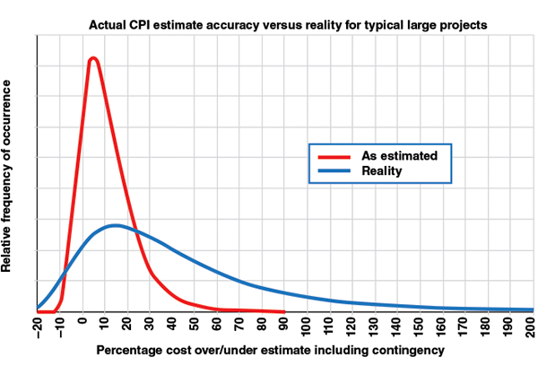
FIGURE 1. In reality, large CPI projects often miss the mark with contingency estimation methods, and large discrepancies between actual and estimated values occur
Quoted ranges in literature, such as ±10% at sanction, typically reflect an estimation of process quality uncertainty, not project risks. These tight ranges reflect the estimator’s and team’s confidence in how well they quantified and priced the given scope. They assume nothing will change, no risk events will occur and that project control will be excellent. Of course, these assumptions are rarely realistic for owners, although they may be somewhat more realistic for contractors, for whom contingency must only cover uncertainty within the contract scope.
Figure 1 is not the only story; there also exists a stark dichotomy in industry estimation practices between small and large projects. Figure 2 depicts an example distribution of accuracy outcomes for small projects in a U.S. plant-based project system, where the project is managed by an operating facility rather than a major projects organization. At the plant level, engineers may also act as estimator and project manager. For small projects, the range is still wide; small projects do not benefit from the balancing of underruns and overruns among a multitude of cost items. However, they are biased much further to the low side. The resulting midpoint is a slight underrun. This usually reflects conservative base estimates with a generous use of “allowances.”
In lean plant-based organizations, where each project leader has many projects of short duration, the emphasis is on getting operations up and running quickly and safely. One cannot spend weeks or months arguing for money to cover an overrun, so projects are frequently overestimated, often subconsciously. If excess money is returned to the business in a disciplined way, like in the example shown in Figure 2, this bias need not be wasteful, although it does lock up capital for some time. Those who understand this behavior will not be surprised that most predictable owner capital-project systems tend to be those that are most accurate. These tight-range systems tend to have an overfunding bias, and they spend the excess, which, on average can be 5–20% more than disciplined, but less predictable, systems.
To summarize the above discussion, there are no standard ranges. Large projects managed by major owner-project groups typically experience greater risk than expected and face greater cost scrutiny, so base estimates are tight and contingency is underestimated. Small projects managed by plants, while having their share of risk, are typically overestimated. So, when it comes to improving accuracy and contingency estimation, one must pay careful attention to the level of scope definition, specific risks and biases. These are discussed in the following sections.
Know your scope
Table 2 illustrates how estimate accuracy improves with the level of scope definition. This is no longer an arguable topic. Since the 1990s, almost every major CPI owner company has implemented a phase-gate project system, and the phases usually line up with the AACE Estimate Classes in Table 2. The topic of scope definition, in terms of knowing which deliverables are important, and how to rate their definition, is well covered in literature. Example rating schemes for the CPI include AACE’s Classes (RP 18R-97), the Construction Industry Institute’s (CII; Austin, Tex.; www.construction-institute.org) Industrial Project Definition Rating Index (PDRI) and IPA, Inc.’s (Ashburn, Va.; www.ipaglobal.com) Front-End Loading Index (FEL). The level of scope definition is the greatest driver of cost uncertainty; understanding that fact is the starting point for analyzing risks.
Other key risk drivers within the project scope include the introduction of new technology in the process and the level of complexity in the physical system, as well as the execution strategy itself. Decades of empirical industry research on the impact of scope definition, technology and complexity on cost accuracy have proven these points (see sidebar on RAND and Hackney). AACE refers to these dominant risk drivers as “systemic” risks because they are intrinsic to one’s project and physical systems.
Know your base estimate
Per Table 1 definitions, the “base estimate” excludes risk — it’s just the facts. Base estimating practices are well covered in literature [3]. Base estimating is essentially the same, whether done by an owner or contractor. Allowances for uncertainty within the base should be used sparingly. They should be limited to specific uncertain line items and well-documented markups — not general uncertainties or risk events. To avoid bias, a company should have an up-front cost strategy stating what the base estimate should represent. For example, if a company’s key performance indicators call for lower absolute capital cost (rather than predictability), a policy may be as follows: “The base estimate and its assumptions will reflect aggressive, but reasonably achievable performance and pricing, excluding all contingency, escalation, currency and reserve risks.”
The base estimate quality and uncertainty depend on the rigor of the project, and the estimating processes and practices that have been applied, as well as the capability and competency of the team and its tools. In addition, estimating relies on an understanding of performance on past projects, so the quality of reference data that are available, such as unit hours, is a base uncertainty driver. These base estimating factors represent “estimating-quality uncertainty,” which is an important risk driver. However, one should remember that accuracy is, for the most part, not a measure of estimate base quality, but of other more dominant risks.
Optimism Bias
Perhaps the most published author on the topic of cost overruns has been Bent Flyvbjerg of Oxford University (Oxford, U.K.; www.oxford.ac.uk). His empirical research on publicly funded infrastructure projects pins the cause of major overruns on optimism bias; and, to the extent that politics and tax or rate payers are involved, on strategic misrepresentation or “lying.” His articles have raised awareness of the cost situation shown in Figure 1. However, his prescription for addressing the situation, called reference-class forecasting (RCF), has been largely one of risk acceptance, where one accepts that optimism bias cannot be effectively countered, and run project economics using historical norms (the RCF) as the most likely outcome. In the CPI, we know there are effective practices, such as phase-gate systems, to improve accuracy, and that the profit motive will temper optimism bias. â‘
Biases and estimate validation
Capital project management is a realm of intense cost pressures and biases. If a high estimate scuttles project sanction, the estimator’s performance rating and career development may be put at risk. In slow economic times, cancellation of a large project may mean the loss of the team’s jobs. For decision makers, optimism bias often prevails. For many reasons, the desire and pressures to make a “go-ahead” project decision can be immense. The more strategic the project, the more these biases create pressure for lower cost estimates, resulting in discrepancies like those seen in Figure 1.
On the other hand, overruns may be punished, and this drives conservative estimating practices by those afflicted, particularly in small project systems (Figure 2). If the strategy is schedule-driven, as is more common in high-margin specialty chemicals or upstream production, there may also be less pressure to minimize costs, while the opposite is true for lower-margin commodity chemicals or petroleum refining.
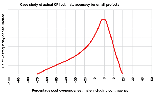
FIGURE 2. This example distribution of accuracy outcomes for small projects shows that excess capital can, in fact, be returned to the organization if disciplined planning and estimation occurs
These biases and their effect on estimating behavior are all major sources of cost uncertainty. If the bias is toward decreased base estimates (see sidebar on optimism bias), more contingency will be required, and vice-versa if the bias is toward increased base estimates (punitive cultures or small projects). In any case, one’s contingency estimation methods must rate and cost these biases.
Unfortunately, bias has a political element, and is therefore very difficult to rate and price objectively. To counter this, benchmarking and quantitative estimate validation are recommended practices that measure bias relative to norms. Preferably, objective third parties will conduct these validation steps.
Estimate validation compares the metrics of an estimate to metrics based on historical data. These metrics are usually ratios of one cost-estimate element to another, such as high-level cost-to-capacity metrics, or more detailed unit hours or unit costs. For example, if the comparable historical actual data for piping installation unit hours ranges from 10 to 18 h/kg, and one has an aggressive target cost strategy, one might expect the base estimate without contingency to be about 10 h/kg, anticipating it will grow to a competitive (perhaps, aggressive but reasonably achievable) 12 h/kg upon completion. Without a cost strategy, estimators who are left to their own devices will tend to use an approach based on “historical norms,” which uses a midpoint of history or experience (14 h/kg in this particular example), which will be biased toward less competitive outcomes, because it presumes risks will happen without actually identifying or quantifying them. In any case, quantitative validation gives one an objective read of the bias, and the subsequent need for contingency.
Identify the risks
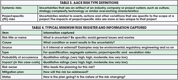
The above discussion covers the rating of what AACE calls “systemic” risks, including the level of scope definition and project system capabilities. Next, one must begin to understand risks that are project-specific (PS). Table 3 provides AACE International’s definitions for these risks types; they are important to understand because the recommended methods for quantifying these risks vary by type. Note that “escalation” is a third type of risk, covering price changes driven by the economy, which should be estimated separately by methods not covered in this article.
The risk-management process starts with identifying the risks on the project. This is usually done in a workshop setting with key stakeholders and members of the project team. Risk identification can also be done via interviews or other means. Often starting with a checklist, the workshop facilitator guides the group through a brainstorming session to identify any threats or opportunities that may result in the project not meeting its objectives. These are captured on a risk register that records key risk attributes and risk-management planning elements. Table 4 shows the minimum information one will want to capture, discuss and record in a typical risk register.
Before quantifying the risks, prioritize them and focus only on those that are critical. Critical risks can create major hurdles to meeting project objectives, in this case costs. To evaluate critical risks, the team agrees to a set of qualitative ratings (very high, high, moderate, low, very low) for probability and impact with associated indicative values. For example, a “very high” rating could represent >5% of total cost and >50% probability. The team then comes to a consensus on the probability and impact ratings for each risk in the risk register. Critical risks are typically in the top category of probability and impact. If risks are well-managed during scope development, there should be very few of these. Figure 3 illustrates a typical five-by-five risk matrix, where red coloring denotes critical risks.

FIGURE 3. A typical probability-versus-impact risk matrix allows for quick visualization of critical risks, and facilitates simpler decision-making
Quantify the risks
Having identified the critical risks, and being at a decision point where contingency must be set, the next step is to quantify the risks. Best practice dictates the use of probabilistic risk analysis to derive a distribution of possible project cost outcomes. With a specific distribution and base estimate value in mind, contingency is simply the cost that must be added to get a desired probability of underrunning the total, as shown in Figure 4. Management will decide on their desired probability. Probability of underrun levels from p50 to p70 are common, depending on how risk-tolerant or risk-averse the company’s management is. Note that contingency has no effect on the project’s cost distribution or absolute cost range. Those are fixed attributes of the project and its uncertainty profile as it stands at that point in time. From the distribution, a worst-case value can also be obtained for sensitivity analysis (for instance, p90).
So how can engineers come up with a probabilistic cost distribution like the one shown in Figure 4? Since the 1980s, when the first Monte-Carlo simulation (MCS) add-on for spreadsheets was introduced, the traditional answer was a method called line-item ranging (LIR). This method involves assigning low and high range values (ends of triangular distributions) to one’s cost-estimate line items, and running the MCS software. However, LIR has been discredited by research. It fails because it violates a first principle of risk analysis; it does not “quantify the risks.” LIR does not make a risk-to-impact link. Teams cannot intuitively, and certainly not item by item, make the risk-to-impact leap. In terms of statistical significance, LIR tends to produce almost the same curve every time it is used — the red curve of Figure 1. Research published by IPA Inc. shows that LIR results in 9% contingency with ±4% standard deviation, regardless of actual risks [4]. The problem is not MCS itself; the problem is that the LIR model only addresses “estimating process quality” risk. However, like a broken watch, it does get the number right occasionally, such as when there are no other project risks.
Without using LIR, what is an engineer to do? Rather than fall back on a rule-of-thumb percentage, AACE recommends several risk-quantification methods that apply first principles in RP-40R-08 [5]. Two methods are readily available, and can be applied without specialized software and training, although, on major projects, using experts for risk analysis is highly recommended. Additionally, these two methods can provide an average contingency value without probabilistic modeling, if desired. These AACE methods are covered in the following RPs:
- 42R-08: Risk Analysis and Contingency Determination Using Parametric Estimating
- 44R-08: Risk Analysis and Contingency Determination Using Expected Value
Two methods are needed because the two very different types of risk, systemic and project-specific, must be addressed. The Parametric Estimating method is used to quantify systemic risks, because their impacts are only knowable through analysis of historical experience. The Expected Value method is used to quantify project-specific risks, because their occurrence and impacts are readily estimable by the team.
The RAND and Hackney Parametric Cost Risk Models
On its website, AACE International provides two working Microsoft Excel models for quantifying systemic risks (RP 43R-08). One model is by the late John W. Hackney, a founder of AACE, as first published in his 1965 landmark text “Control and Management of Capital Projects,” the 2nd edition of which is now published by AACE International. Hackney studied actual projects from his experience, and developed an elaborate contingency model based on the rating of many systemic risk factors. In 1981, the RAND Corp. (Santa Monica; Calif.; www.rand.org) published a groundbreaking report entitled “Understanding Cost Growth and Performance Shortfalls in Pioneer Process Plants” (Rand R-2569-DOE). That report includes an empirically based parametric model of cost growth, including statistical parameters. The study’s lead author, Edward Merrow, went on to found IPA, Inc., and Hackney was a consultant to the 1981 study. These two publications should be on every CPI cost estimator’s bookshelf. â‘
Quantification: point value only
Parametric estimating uses a pre-determined equation in which the predicted average contingency percentage (to apply to the base estimate) is the equation outcome (the dependent variable), and numeric ratings of the systemic risks are the inputs (the independent variables), as shown in Equation (1).
MSC, % = Constant + A × (SDR) + B × (CR) + C × (EBR) + (OR) (1)
Equation (1) follows a typical parametric model or output of a regression analysis in the following form: Value = constant + coefficient A × parameter A + coefficient B × parameter B, and so on. In this case, to obtain the mean systemic-risk contingency (MSC) percentage value, the parameters are quantified values of scope definition rating (SDR), complexity rating (CR), estimate bias rating (EBR) and the product of any other coefficients and systemic risk ratings (OR). A, B and C are the respective coefficients, which along with the regression constant, are developed from regression analysis of historical data or published models in literature.
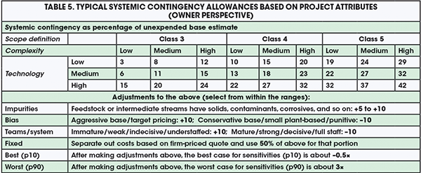
All the team has to do is rate their project’s systemic risks and bias, and insert the ratings into the equation. The challenging part is developing a risk-rating scheme and an equation. Most companies do not have historical cost and risk data with which to develop an equation using regression analysis. Fortunately, rating schemes and reliable equations are available, based on 50 years of CPI research. Two time-honored rating schemes and equations are built into working Microsoft Excel tools, which are publicly available on AACE’s website, and documented in RP 43R-08 (see sidebar on RAND and Hackney). For those looking for a quicker answer, Table 5 provides systemic contingency values similar to the RAND model, but instead applies a model derived by the author.
The values in Table 5 are average allowances (about p55). They assume a large gas or liquids CPI project with 20% equipment cost and typical project-management system maturity and biases. For Class 3 scope definition, it assumes that 5% of the total cost has already been spent on engineering, and that the class is over-rated. Few projects achieve ideal Class 3; most are funded closer to Class 4. As seen in Table 5, a wide range of complexity is taken into account, with low-complexity projects having less than three block-flow process steps with a simple execution strategy, and high-complexity projects having more than six continuously linked process steps or a complicated execution strategy. The technology basis varies from less than 10% of capital expenditure (capex) for a process step with commercially unproven technology to greater than 50% of capex for new, R&D or pilot scaleup steps. Engineers can make adjustments to the indicated table value as shown. The fixed-price adjustment allows for less uncertainty for that element, but there is no such thing as fixed price for owners; change and risk events will inevitably happen. Per the precedents in Table 5, an example of best/worst case (p10/p90) application is as follows: if systemic contingency is +10% (Class 4, low complexity, no new technology), the corresponding best and worst cases would be –5% (–0.5 × 10) and +30% (3 × 10), respectively. Note that the best case under-runs the base estimate in this scenario.
After quantifying the systemic risks, the Expected Value method is used for each critical project-specific (PS) risk to determine the average contingency cost to add to the base estimate. The exception is for Class 5 estimates, for which specifics are unknown and systemic contingency can be used alone. If risks have been largely mitigated during early design, and risk screening is done correctly, there will typically be less than 10 critical project-specific risks. Never quantify all of the risks in a register, of which there may be hundreds — the systemic allowance covers typical risk “noise” for non-critical risks. The simple Expected Value expression for determining the mean PS contingency value (MPSC) percentage is shown in Equation (2), as the summation of the products of probability of risk occurring (Prisk) and the cost impact (in $) if the risk occurs (CI).
MPSC = ∑(Prisk × CI) (2)
Consider that a workshop is held in which key team members rate the systemic risks for application of Table 5 and then discuss the critical risks and quantify their probability and most likely impacts if they occur. For example, assume the team estimates there is a 20% chance that the project will encounter rock requiring blasting in the soils during foundation excavation, and the most likely cost for this was $50,000. If the cost of rock-blasting was <1% or so of the base estimate, it probably would not constitute a “critical” risk and the team would move on to the next risk. If it was critical, say 20% probability, then the expected value to include in the contingency sum would be 0.2 × $50,000 = $10,000. Another consideration is whether this risk is a binary, discrete or overwhelming risk.
The Expected Value method works best for risks with a continuous range of impacts. In this case, the rock blasting could be $1,000 to $100,000 depending on severity. But if the impact is all-or-nothing, there is no point in putting a percentage of the impact in contingency. These types of risks should be presented to management as possible “management reserve” items that they may wish to fund in their entirety (or not) with the funds to be disbursed to the team only if the risk occurs. Using this approach, the total mean contingency is the sum of the two parts, as shown in Equation (3).
Ctotal = (MSC × BE) + ∑(MPSC) (3)
This equation calculates a total (mean) contingency cost (Ctotal, in $). It is the sum of MSC from Equation (1) times the base estimate cost (BE), and the summation of the mean PS contingency values for each of the PS risks from Equation (2).
For example, if the systemic contingency was 10%, the base estimate was $1,000,000, and the sum of the PS risk expected values was $50,000, the total contingency would be 0.1 × 1,000,000 + $50,000 = $150,000. Again, the corresponding worst-case value for business-case analysis would be three times this amount.
Full cost distribution
The two methods above produce a point value and worst-case for contingency. However, the best practice, as shown in Figure 4, is to develop the full cost distribution so that management can select contingency and worst-case values depending on their level of risk tolerance. This can be done using inferential statistics applied to the Parametric Estimation model, along with MCS applied to the Expected Value method, with the parametric outcome included as risk number one. For this, one must have an MCS add-on to Microsoft Excel, such as @RISK, available from Palisade Corp. (Ithaca, N.Y.; www.palisade.com), or Crystal Ball, available from Oracle Corp. (Redwood Shores, Calif.; www.oracle.com).
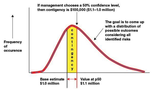
FIGURE 4. A probabilistic cost distribution can be used to determine contingency
MCS application description is beyond the scope of this article. However, for those with knowledge of the practice, a simple MCS model can be developed by applying MCS to Equation (3). This is done by replacing the systemic contingency percentage and each PS risk-impact estimate in the worksheet with distributions per the software procedure, and simply running the simulation. The Table 5 method provides the most-likely, and p10/p90 values for systemic contingency percentage. The team, in their project-specific risk workshop, will not only estimate the most likely impacts, but the low and high range as well. The MCS software will generate a distribution similar to that in Figure 4.
Communicating the risks
Contingency is one of the most controversial topics for CPI capital-project management. Every stakeholder on the team has a different perspective as to what contingency represents, the extent to which it is necessary, and how it should be managed. This article assumes that the owner company agrees with the AACE definition; that contingency is expected to be spent. They also practice disciplined management of change on their projects. They understand that for a safe and cost-effective project, contingency under the authority of an experienced project manager is necessary to respond to risks in near realtime. Delays in response, such as requiring a committee or senior manager to review all contingency use, often result in the compounding of risk impact. The engineer must communicate this point of view to those responsible. Any distortion of these conditions will result in contingency being something other than what is described here, and its quantification tends to become more of a game.
If the company shares a common view about contingency, then communication can focus on making sure that management understands the risks’ drivers and their relative impacts. Per Figure 4, contingency is selected by management decision-makers based on their risk tolerance. Ideally, risk-analysis will be done well ahead of the funding decision, so that the team has time to recycle plans to manage risks and impacts that are found to be unacceptable. The methods in this article facilitate risk communication and treatment because they are risk-driven, meaning that the risks and impacts are explicitly linked.
Edited by Mary Page Bailey
References
1. AACE International, RP-10S-90: Cost Engineering Terminology, Jan. 2014.
2. AACE International, RP-18R-97: Cost Estimate Classification System — As Applied in Engineering, Procurement and Construction for the Process Industries, Nov. 2011.
3. Dysert, L., Sharpen Your Capital-cost Estimation Skills, Chem. Eng., Oct. 2001.
4. Merrow, E., “Industrial Megaprojects,” John Wiley & Sons Inc., New York, N.Y., 2011.
5. AACE International, RP-40R-08: Contingency Estimating: General Principles., June 2008.
Author
 John K. Hollmann is the owner of Validation Estimating, LLC (21800 Town Center Plaza, Suite 266A-180, Sterling, VA 20164; Email: [email protected]; Phone: 703-945-5483). With 37 years of experience in design engineering, cost engineering and project control, including expertise in cost estimating and risk analysis for the process industries, Hollmann is a life member and past board member of AACE International. He was editor and lead author of AACE’s technical foundation text, “Total Cost Management Framework” (2006). Hollmann has a degree in mining engineering from the Pennsylvania State University and an MBA from the Indiana University of Pennsylvania. He is a registered professional mining engineer in the state of Pennsylvania and holds the following AACE professional certifications: Certified Cost Professional, Cost Estimating Professional and Decision and Risk Management Professional.
