Gas compressibility can lead to choked flow in piping systems. Presented here is an overview of choked-flow geometries in pipes, and examples of how choked flow arises in different pipe layouts
The more things change, the more they stay the same. At least that is how the saying goes. What has changed? The chemical process industries (CPI), along with industry more generally, continue to evolve and expand the importance and breadth of fluid-system applications. And what has stayed the same? The phenomenon of sonic choking in superheated gas flow remains a challenge in process piping applications.
Sonic choking occurs when gases, which are compressible, flow at velocities that approach sonic velocity, the speed of sound waves in a medium. A typical sonic velocity for air is 1,000 ft/s (305 m/s). When a flowing gas at some location in the pipeline experiences a local velocity equal to the sonic velocity of the gas at that temperature, sonic choking occurs.
Twenty-five years ago, an article was published in Chemical Engineering entitled “Gas-flow Calculations: Don’t Choke” [1] (Figure 0). This article revisits the material in the piece from 2000, providing clarifications, updates, points of emphasis and additional insights from the author’s experiences over the last quarter century.
FIGURE 0. The cover of the Chemical Engineering issue from January 2000 is shown here, featuring the author’s original article, as cited in Ref. 1
Another impetus for this revisit article is that the author recently wrote a technical paper that details all the types of sonic choking [2]. This included discussion of multiple sonic choking points in series and in parallel. In doing so, examples of all these situations were created using simplified assumptions, such as assuming perfect gas and adiabatic flow in horizontal pipes. This allowed the examples to be solved using closed-form solutions and applied in Microsoft Excel. The Excel files are publicly available [3] for those interested and examples are included here.
The goal of the present article is not to just repeat discussions from Ref. 1. Rather, the purpose is to offer some clarifications and reinforcements to the previous article. And the Excel-based examples from Ref. 2 will be used to provide a hands-on, accessible learning tool for those interested in a deeper dive.
Even though a quarter century has passed, the author continues to see engineers trying to use incompressible-flow methods on compressible-gas systems and using or promoting the debunked “40% pressure drop rule.” Please consult Ref. 1 for a thorough explanation of why “rules of thumb” like this and other similar ones can be highly misleading. Finally, guidance is provided for what to look for when evaluating software for modeling pipe systems where sonic choking might occur.
Quick review of sonic choking
Sonic choking occurs when the gas bulk velocity reaches the gas sonic velocity somewhere in a pipe system. This is another way of saying that the Mach number reaches 1. When this happens in a sequential run of pipes, then lowering the downstream pressure will not produce any additional flow. Figures 3 and 4 from Ref. 1 and the associated discussion there do a good job of elaborating. Further discussion on sonic choking can also be found in Ref. 2.
When the first article was published in 2000, the author was under the impression that a sonic choking point involved a shock wave. After discussions of this concept with several other knowledgeable engineers over the years since the publication, he is now unsure of this, and has stopped calling it a shock wave. Regardless, a sonic choking point is (at minimum) similar to a shock wave in that it involves a discontinuity in the flow field. Therefore, whether or not there is a shock wave is somewhat irrelevant. A discontinuity exists, and that is what is important.
Geometry of sonic choking
Both Refs. 1 and 2 discuss in depth the three geometric situations where sonic choking occurs. Because the examples from Ref. 2 to be explored here are designed to examine all the possibilities of these three geometries, including cases where two, or all three, geometries are happening in the same system, the three situations are discussed here.
1. Endpoint choking (Figure 1, top diagram). Endpoint choking occurs when the gas pressure in the pipe cannot drop down to the discharge pressure without accelerating to sonic velocity thereby resulting in a choke point (and pressure discontinuity) at the end of the pipe.
2. Expansion choking (Figure 1, middle diagram). Expansion choking occurs when there is an increase in pipe area, such as an expander, diverging tee, or discharge into a large header pipe. Here, the gas cannot navigate to the pipe discharge downstream without accelerating to sonic velocity at the point where the area increases. A choke point and pressure discontinuity thus occurs.
3. Restriction choking (Figure 1, bottom diagram). Restriction choking occurs when there is restriction (resultting from an orifice or valve, for example) where the gas cannot navigate through the restriction without accelerating to sonic velocity. A choke point and pressure discontinuity thus occurs at the restriction.

FIGURE 1. Each of these pipe configurations can result in sonic choking
Solvable boundary conditions
In a sequence of pipes, there are three types of solvable boundary conditions [2], as depicted in Figure 2. Repeateed reference to Figure 2, diagrams A, B and C will be made throughout the following seven examples in order to point out which part of the choked pipe system is solved with which combination of boundary conditions.
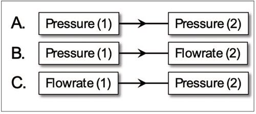
FIGURE 2. The diagram here shows types of solvable boundary condition combinations for a pipe or pipe sequence (flow from left to right)
Important equations
A form of the mass-conservation equation is highly useful for gas-flow calculations in pipes, in general, and for sonic-choking calculations specifically (Equation (1) [1, 2]).
![]()
(1)
Because choked flow occurs when the Mach number equals 1, Equation (1) becomes Equation (2).
![]()
(2)
A closed-form solution of adiabatic flow in constant-diameter pipes can be found in most compressible-flow textbooks where the pipe is horizontal with a constant friction factor (Equation (3) [1, 2]):
![]()
(3)
Note that Equation (3) is sometimes presented without all the parenthetical groupings, which can be misleading. For example, the author did this in Equation 11 from Ref. 1. The Equation (3) form here is preferred because it makes clear the otherwise ambiguous parenthetical groups. Equations (1) to (3) are applicable for real gases.
Preface to all examples
In order to provide closed-form solutions in Microsoft Excel, simplifying assumptions are required. All examples assume the flowing gas is air, follows the ideal gas law, is calorically perfect, with an isentropic expansion coefficient of 1.4. All pipes are assumed to be adiabatic, constant-diameter and horizontal, which allows Equation (3) to be used. Entrance losses are ignored.
Including real-world behavior, such as heat transfer, real gas behavior, sloped pipes and varying friction factors, is important and will be discussed in a subsequent section.
Space limitations do not allow a thorough discussion of all examples, so brief information will be given about each one. Refer to Ref. 2 for more details.
Single-choke-point examples
Example 1: Endpoint choking, single choking point. Figure 3 (top) shows the input for Example 1, endpoint choking, and Figure 3 (bottom) shows the output. Here, the Figure 2a boundary condition combination is used. From Figure 3 (bottom), any discharge pressure at or below 95.3 psia (657.1 kPa) will result in choking.
Example 2: Expansion choking, single choking point. Figure 4 (top) shows the input for Example 2 (expansion choking), and Figure 4 (bottom) shows the output. The input data for Pipe 1 is the same as for Example 1. Here, the Figure 2a boundary condition combination is used for Pipe 1. How is Pipe 3 solved? Once the choked flowrate is determined for Pipe 1, that becomes a known boundary condition to use for the inlet of Pipe 3. Hence, Pipe 3 is solved using the Figure 2c boundary-condition combination. From the Law of Conservation of Mass, the mass flowrate in Pipe 3 is the same as that in Pipe 1. Further, from the energy conservation law, the stagnation enthalpy at the inlet of Pipe 3 must match the outlet of Pipe 1 [2] regardless of whether the pipes are adiabatic or not.
Example 3: Restriction choking, single choking point. Figure 5 (top) shows the input for Example 3 (restriction choking) and Figure 5 (bottom) shows the output. The input data for Pipe 1 is the same as Example 1. Here, the Figure 2a boundary condition combination is used for Pipe 1. Once the choked flowrate at point J2 is determined, that becomes a known boundary condition to use for the inlet of Pipe 2. Hence, Pipe 2 is solved using the Figure 2c boundary condition combination. Similar to Example 2, mass and energy conservation across J2 will determine the mass flowrate and stagnation enthalpy at the inlet of Pipe 2.
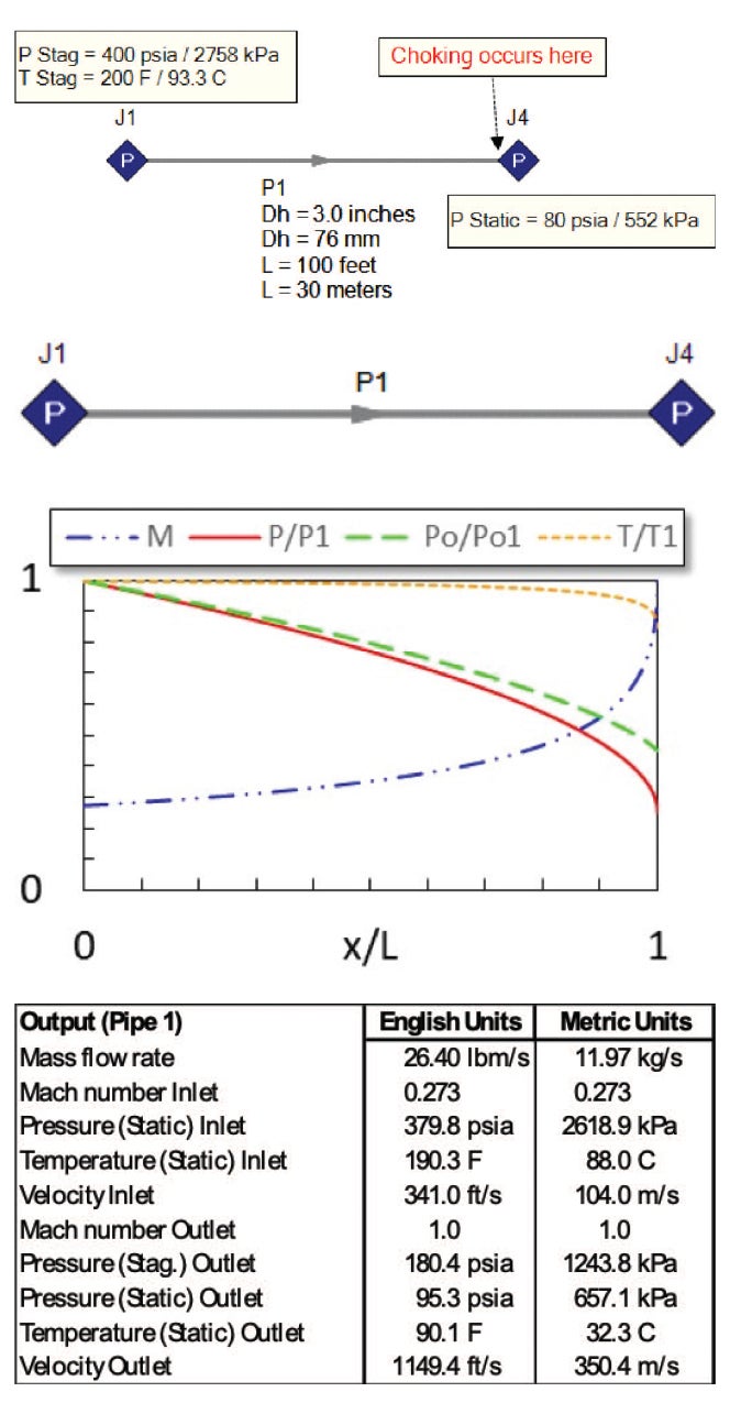
FIGURE 3. Endpoint choking input data (top) and output data (bottom) are shown for Example 1
Multiple choke points in series
Example 4: Two choking points in series with expansion choking first. Example 4 is similar to Example 2 (Figure 4, top), except for one change. The downstream pressure is reduced from 100.6 psia (693.5 kPa) to 50 psia (344.7 kPa). Figure 6 (top) shows the input. This results in endpoint choking occurring at point J4. Hence there are two sonic choking points. Figure 6 (bottom) shows the output. Similar to Example 2, the Figure 2a boundary condition combination is used for Pipe 1 and the Figure 2c boundary condition combination is used for Pipe 3. Mass and energy conservation across J3 determine the conditions at the inlet of Pipe 3, similar to Example 2.
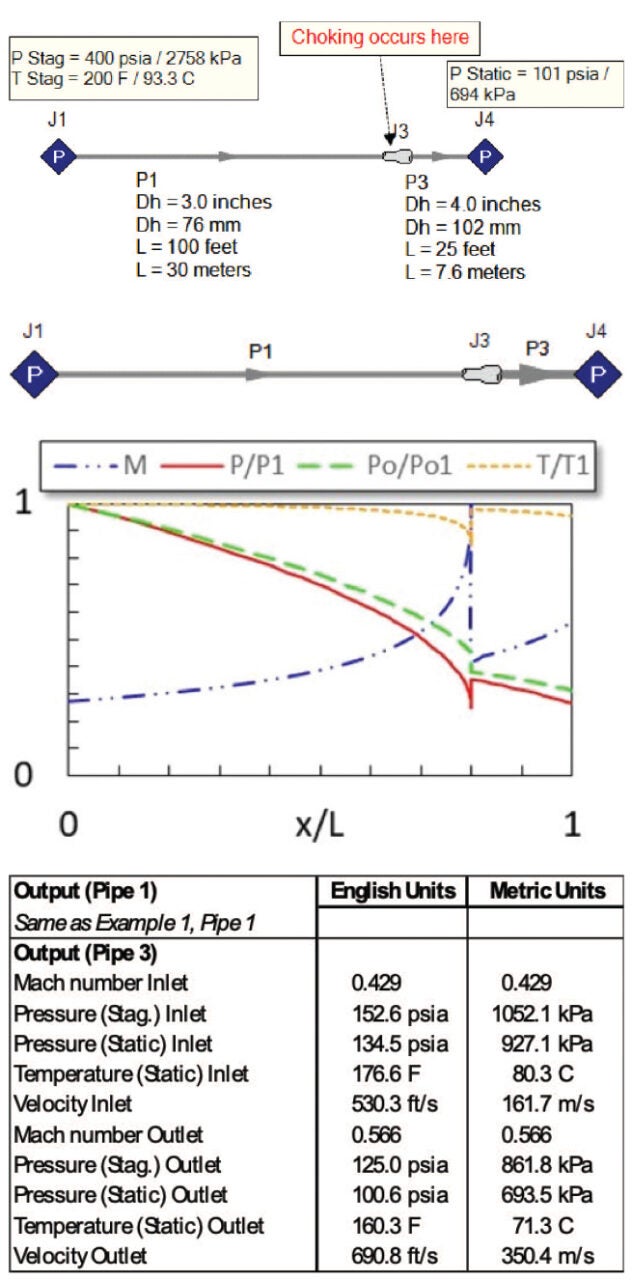
FIGURE 4. Expansion choking input data (top) and output data (bottom) are shown for Example 2
Example 5: Two choking points in series with restriction choking first. Example 5 is the same as Example 3 (with Figure 5, top), except with one change. The downstream pressure is reduced from 100.6 psia (693.5 kPa) to 50 psia (344.7 kPa). Figure 7 (top) shows the input. This results in endpoint choking occurring at J4. Hence, there are two sonic choking points. Figure 7 (bottom) shows the output. Similar to Example 3, the Figure 2a boundary condition combination is used for Pipe 1 and the Figure 2c boundary condition combination is used for Pipe 2. Mass and energy conservation across J2 determine the conditions at the inlet of Pipe 2, similar to Pipe 3 in Example 3.

FIGURE 5. Restriction choking input date (top) and output data (bottom) are shown for Example 3

FIGURE 6. Expansion choking input data (top) and output data (bottom) are shown for Example 4, for two choking points in series, with expansion choking first

FIGURE 7. Restriction choking input data (top) and output data (bottom) are shown for Example 5 for two choking points in series
Example 6: Three choking points in series. Figure 8 (top) shows the input for this example. This situation results in restriction choking at J2, expansion choking at J3 and endpoint choking at J4. Hence, there are three sonic choking points. Figure 8 (bottom) shows the output. The Figure 2a boundary condition combination is used for Pipe 1 and the Figure 2c boundary condition combination is used for Pipe 2 and, again, for Pipe 3. Mass and energy conservation across J2 and J3 determine the conditions at the inlet of Pipe 2 and Pipe 3, similar to previous examples.

FIGURE 8. Input data (top) and output data (bottom) are shown for Example 6, for three choking points in series
Multiple choke points in a sequence of pipes
When there is more than one choking point in a sequence of pipes, the first choking point controls the mass flowrate for the entire sequence. While the choking points downstream do not control the flowrate, they do control how the pressure is distributed and, hence, the pressure profile. For example, consider Figure 8 (bottom) from Example 6. The first choking point here is at the J2 restriction choking point, and this controls the flowrate (14.74 lbm/s/6.69 kg/s). The J3 and J4 choking points control how the profile graphs appear in Figure 8 (bottom) downstream of J2.
Multiple choke points in parallel
Example 7: Four choking points in parallel flow paths. Figure 9 (top) shows the input. This results in restriction choking at J12 and J22, and endpoint choking at J13 and J23. Hence, there are four sonic choking points. Figure 9 (bottom) shows the output, which is more complicated than previous examples because of the flow split at J11 and the parallel paths. Also, the two choked-flow paths are non-symmetrical (Figure 9, top) and, hence, have different flowrates. The Figure 2a boundary-condition combination is used for Pipe 1, Pipe 11 and Pipe 21. The Figure 2c boundary-condition combination is used for Pipe 12 based on the choked flow in the J12 orifice, and for Pipe 22 based on the different choked flow rate in J22 orifice.
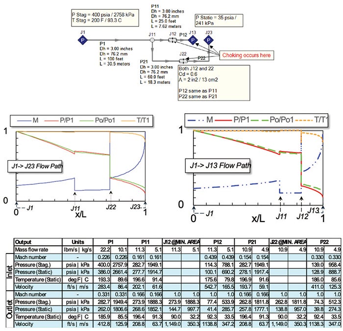
FIGURE 9. Input data (top) and output data (bot-tom) are shown for Example 7, for four choking points in two parallel flow paths
Mass and energy conservation across J12 and J22 determine the conditions at the inlets of Pipe 12 and Pipe 22, similar to previous examples. While this example could be solved in Excel using excessive manual iteration for the conditions at J11, this was skipped, and results came from the commercial software AFT Arrow [4]. Note that in Ref. 1, version 2 of the software was used, but for this exercise, version 10 was used.
Finally, if conditions were right, one more choking point could exist in this system. This would be at the J11 node, which expands into P11 and P21. It is possible for expansion choking to exist at the end of Pipe 1 here. This would occur, for example, by reducing the diameter of Pipe 1 to 2 in (51 mm) and reducing the pressures at J13 and J23 to 15 psia (103 kPa). This would result in 5 choking points in Figure 9a.
Downstream of choke points
Many conditions exist downstream of choke points that process engineers may need to know. Among these is to understand how the flow of gas will distribute to parallel delivery points and what the process conditions are at those delivery points. A more complete list of these conditions can be found in Section 6.5 of Ref. 2.
Application of Equation (2)
In order to correctly determine the choked flowrate, Equation (2) must be applied at each local choke point. That means that for each of the examples presented, accurate knowledge of the stagnation pressure and temperature, Po, and To, must exist at each local choke point. When conditions are ideal, like the examples presented here, it is more straightforward to determine these conditions using equations such as Equation (3). However, when real-world conditions must be accounted for, it is quite complicated to determine Po and To at each choke point. Indeed, determining these values depends on knowing the mass flowrate — which is the variable for which we are solving. In such cases, heavy numerical iteration is needed using the governing conservation equations. The original article [1] discusses these in more detail.
Simplified to complicated
Simplifications such as Equation (3) and the examples presented here are useful to gain an appreciation of how to navigate single or multiple sonic choking points — and how to determine conditions downstream of choke points. In most real systems, Equation (3) will not get you far. Real-world effects, such as heat transfer between ambient surroundings and the gas will need to be accounted for. Other effects include real gas behavior, sloped or vertical pipes, variable friction factors and complex pipe networks. A capable software tool that accounts for all these effects is essential to obtain accurate predictions in such situations [4].
Do you know what γ (or k) is?
The isentropic expansion coefficient is commonly called γ by gas dynamicists (or k by thermodynamicists). In engineering school, the author learned the following relationship, shown in Equation (4):
![]() (4)
(4)
However, a little-known fact [5] is that Equation (4) is actually an approximation, and is the simplified form of the full definition of γ, as shown in Equation (5):
![]() (5)
(5)
It is often the case that the “correction term” on the righthand side of Equation (5) is close to unity, thus making Equation (4) approximately correct. On the other hand, the author has found that the complete Equation (5) is commonly required in gas-pipe analysis in order to obtain accurate results.
Part of the reason for discussing this here is that after Ref. 1 was published in 2000, there was a respectful, but critical, letter to the editor in a subsequent issue specifically about the assumptions in the 2000 article. An exchange of letters occurred, where Equation (5) was offered as being preferred to Equation (4), which satisfied the critic that the assumptions used in Ref. 1 were, in fact, sound.
Sonic choking analysis software
In order to accurately predict sonic choking in pipe systems, software solutions should be able to handle all types of sonic choking, including multiple choking points in series and parallel. Further, a proper energy balance should be performed on the pipes and choke points. Features such as heat transfer, sloped pipes and real-gas modeling is recommended. For a complete list, see Section 9 in Ref. 2.
Corrections to Ref. 1
The revisiting of the 2000 sonic choking article allows us to correct some typographical errors in Ref. 1 that I found after publication. All errors were the fault of the author.
Equation (14c) in Ref. 1 should have a negative sign, as shown in Equation (6).
(6)
Equation (14e) in Ref. 1 should read, as follows in Equation (7).
![]()
(7)
Concluding remarks
Important concepts from a 25-year-old article in Chemical Engineering are clarified and reinforced. The seven simplified examples in this article demonstrate all the different types of sonic choking configurations with closed-form solutions in Excel. Accounting for real-world gas-flow effects (such as heat transfer) is crucial to obtain accurate predictions. Advice on evaluating commercial software for compressible flow analysis is given. Engineers are cautioned to question common compressible flow calculation “rules of thumb,” such as the so-called “40% pressure drop rule.” Other “rules of thumb” that often lead to confusion are found in the original article.
Edited by Scott Jenkins
References
1. Walters, T. W., Gas-flow Calculations: Don’t Choke, Chem. Eng., January 2000. [PDF of original paper can be found here]
2. Walters, T. W., A Comprehensive Discussion of Sonic Choking In Pipe Systems For Steady, Compressible Flow, presented at the 2024 ASME Pressure Vessel and Piping Conference, PVP2024-123592, July 28 to August 2, 2024.
3. Walters, T.W., A Comprehensive Discussion of Sonic Choking In Pipe Systems For Steady, Compressible Flow, auxiliary data files, https://www.aft.com/technical-papers/a-comprehensive-discussion-of-sonic-choking-in-pipe-systems-for-steady-compressible-flow (2024).
4. AFT Arrow 10, Applied Flow Technology, Colorado Springs, Colo., 2024.
5. Bejan, A., “Advanced Engineering Thermodynamics,” 4th Ed., 2016, pp. 169–170.
Author
 Trey Walters, P.E., is the founder and chairman of Applied Flow Technology (AFT; 2955 Professional Place, Colorado Springs, CO 80904; Phone: 719-686-1000; Email: treywalters@aft.com). His role today is working with AFT team members and customers to deliver industry-leading fluid-transfer-system simulation solutions. He has developed commercial software products on a variety of fluid system applications including compressible flow in pipe network systems. He has managed and performed consulting projects in numerous process industries. He holds B.S. and M.S. degrees in mechanical engineering from the University of California, Santa Barbara. He is a Fellow of the American Society of Mechanical Engineers (ASME).